
Summary
A study on the use of artificial intelligence (AI) in medical image analysis is discussed in the project. Challenges in using AI for medical image analysis, including the need for large amounts of high-quality data and the complexity of the diagnostic process, are mentioned. A dataset provided by the Ministry of Health, which included CT scan images from 1,182 patients, containing a total of 357,405 image slices, was used in the study. The images were divided into 17 different classes, each representing a different health condition. The number of classes was reduced to seven by combining some and removing others.
Convolutional neural networks (CNNs) were used to analyze the images and classify them into their respective health conditions. The CNNs were trained on a subset of the dataset and tested on the remaining images. The authors report that their approach achieved high accuracy in classifying the images, outperforming previous studies on the same dataset.
It is suggested that their approach could be used to assist radiologists in diagnosing health conditions more accurately and efficiently. However, it is also cautioned that further research is needed to validate the approach and ensure its safety and effectiveness in clinical settings.
1. Methods
- Yolo
In our research on YOLO architecture, we found that this architecture is a method that uses convolutional neural networks (CNNs). One of the important features of convolutional neural networks is reducing the number of parameters, which drew our attention to this method. The reduction in parameters causes the model to produce results faster, making the YOLO architecture one of the models we can use well. The YOLO architecture provides us with speed, high success rate, and excellent learning capacity. Additionally, with the bounding box regression and intersection over union (IoU)-based loss function in YOLOv4, the learning capacity of the model improves. As a result, it has been determined that the model will be successful in classification and localization. - Resnet
In our research on ResNet architecture, we realized that it is quite difficult to train very deep neural networks due to the problem of vanishing/exploding gradients. However, the ResNet building block structure allows us to create deeper layer neural networks, solving this problem. Therefore, we decided to use ResNet in our model, thinking that it would increase the model's success by going deeper and extracting more features.
2. Approches
When we reduced the dataset provided to us by the Ministry of Health to a size that could be processed in memory, we noticed that many of the features of the tomography image were lost. We investigated a method of using a "data generator" class, which would allow us to read the images while they were in motion when they were used for training. By reading the images while they were in motion, we saved memory. We customized this class structure by adding various functions such as image preprocessing layers and converting the tomography image to an array by using DICOM.
We had a difficult time deciding between the YOLOv4 and ResNet models we were considering using. Both models had similar success rates. We had read in several articles before that another model was used as a backbone in YOLO and then YOLO classification was done. Based on our tests and observations, we discovered that the ResNet50 model was a good feature extractor. As a result, we decided to use a YOLO model with ResNet50 as the backbone. We created the model architecture again by using the ResNet50 model in the part of the YOLO model that extracts features. We can see this in Figure I.
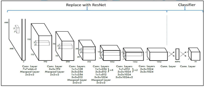
Figure I: Illustration of the part where ResNet will be added on the YOLO model[3]
After completing the model architecture, we changed the default parameters on the model to make it better able to recognize the training set given to us. Instead of using Tanh and sigmoid functions for activation functions, we used a combination of ReLU and Mish functions. This allowed us to avoid the problem of vanishing gradients that can occur in deep-layer models. While ReLU reduced the computational complexity and made the optimization process much faster, Mish increased the model's information storage and discriminative capacity. [4] The reason for this is that Mish has negative derivatives at some points and positive derivatives at others, rather than having all positive or all negative derivatives. [5]
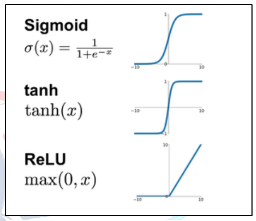
Figure II: Graphs of activation functions
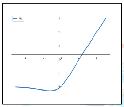
Figure III: Graphs of Mish activation functions
3. Results and Review
There are three successful approaches of the ResNet model, which are ResNet50, ResNet101, and ResNet152. In the given data, only labeled data was randomly split into an 80-20 ratio. The split data was tested with 50 epochs, batch size of 64, categorical cross-entropy as the loss function, and Rmsprop as the optimization algorithm. The results of the tests are shown in Table 1.
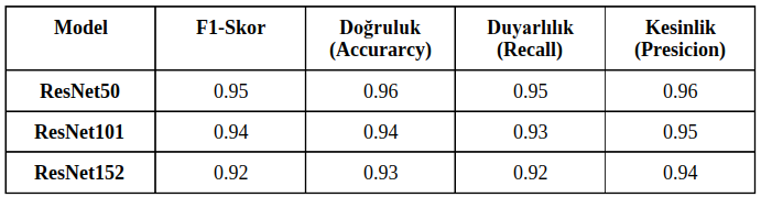
Table I: Comparison of ResNet models on different success metrics
Upon examining Table 1, it is observed that the model that performed the best was ResNet50. The highest training success rate we achieved from the models was calculated as 96.4%. The success metrics of the ResNet50 model, which achieved the best performance, are shown in the training graph in Figure IV, and the model's test results and table are shown in Figure V.
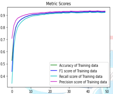
Figure IV: Training graph of the performance metrics of the ResNet50 model
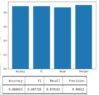
Figure V: Test results and table of the ResNet50 model
Different variations of ResNet, from the original to fully pre-activated, were used on ResNet50 so that the gradients can continue to flow without being blocked by shortcut connections to any previous layers [6]. The reason for using this approach is to enable the model to extract more features without memorization. Subsequently, we removed the classifier layers of the ResNet50 model, making it a pure feature extractor. This approach has been supported by many articles, stating that ResNet is a successful feature extractor. Then, the YOLOV4 classifier layers were used to complete the model. To combine these two models, we used the open-source neural network framework called darknet, written in the C language.
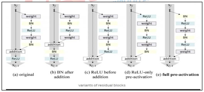
Figure VI: Different residual block variants of ResNet
The YOLOV4 classification layer was connected to the last convolutional layer of the ResNet50 model. We used the loss function of YOLOv4, which is based on classification, confidence, and IOU. This enabled the model to be trained more effectively for both classification and localization.
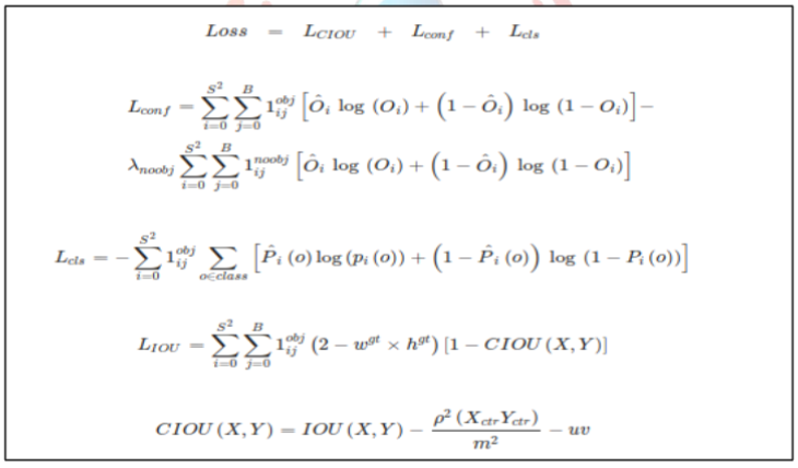
Figure VII: YOLOv4 loss function
After completing the architecture of our model with Resnet50 backbone and YOLOv4, the labeled data provided to us for model training was gathered by only taking the bounding box values from the Excel file. Later, the MBB coordinates were rescaled and adapted to the model for YOLO.
The organized data was divided into 80-20 for training and testing respectively. Additionally, since there was no label of '0' (no detection) in the organized data file, a portion of the test data was added with no detections in a 1/7 ratio.
When selecting hyperparameters for YOLOv4, various tests were performed in many different scenarios. The learning rate parameter was the most important parameter in these tests. Tests were performed with a learning rate of 0.1, then with 0.01, and finally with 0.01, 0.001, and 0.0001 for different training tests. After these tests, we decided that the most suitable parameter for our model was 0.001. Afterwards, we decided on the other parameters based on our research. The hyperparameter selection stage will continue until the day of the competition, and tests will be continuously performed during this process, and our model will be constantly updated. After determining the hyperparameters in our model, we proceeded to the training phase. The best weights during the model's training were saved every 1000 iterations. The loss and mAP graphs for the model can be seen in Figure VIII.
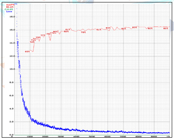
Figure VIII: YOLOv4 training mAP and training loss values
After training the model, the best weights obtained were tested and the mAP result we obtained was 80.73%. The detailed values of the test performed can be seen in Figure IX.
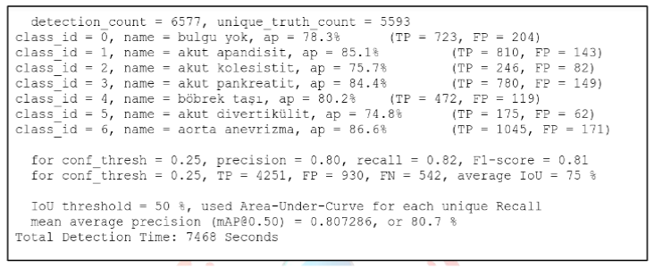
Figure IX: YOLOv4 training mAP and training loss values
4.The datasets used in the experimentation and training phases
Initially, we thoroughly examined the data provided to us by the Ministry of Health. The dataset provided by the Ministry of Health includes the computed tomography (CT) images of 1,182 individuals. There are a total of 357,405 slices in these images, of which 38,236 slices are marked and 5,348 consist of start/end slices. The start/end slices do not have coordinates.
The first shared dataset contains 17 different classes. Each of these classes contains a different number of CT slices. The abdominal aortic aneurysm class has 9009 slices, the acute pancreatitis class has 7121 slices, the acute appendicitis class has 5991 slices, the acute cholecystitis class has 5153 slices, the kidney stone class has 2042 slices, the gallbladder stone class has 1684 slices, the acute diverticulitis class has 1152 slices, the kidney-bladder class has 876 slices, the abdominal aorta class has 852 slices, the abdominal aortic dissection class has 814 slices, the ureter stone class has 726 slices, the colon class has 688 slices, the pancreas class has 632 slices, the gallbladder class has 594 slices, the appendix class has 468 slices, the appendicolith class has 359 slices, and the calcified diverticulum class has 75 slices.
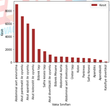
Figure X: Data set distribution graph
As there are too many classes in this dataset, which could complicate the procedures we will perform, we made some changes to the dataset. We removed some classes and merged some others. The organized dataset contains 36,119 marked slices, of which 5,191 are start/end slices. This dataset contains 7 different classes. The "no finding" class has 4111 slices, the acute appendicitis class has 5991 slices, the acute cholecystitis class has 5153 slices, the acute pancreatitis class has 7121 slices, the kidney stone class has 2768 slices, the acute diverticulitis class has 1152 slices, and the aortic aneurysm class contains 9823 slices.
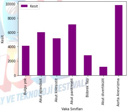
Figure XI: Edited dataset graph
Project information
- Project Name: Computer Vision-based Disease Detection for the Abdominal Region
- Project Category: Deep Learning
- Project date: 01 July, 2022